Reconstruction over a smaller domain using GraphEM

Expected time to run through: 10 mins

This tutorial demonstrates how to get a reconstruction over a smaller domain (30N-70N, 130W-70W) using GraphEM, leveraging HadCRUT4 and the PAGES2k proxy database.

Test data preparation

To go through this tutorial, please prepare test data following the steps:

Download the test case named “PAGES2k_HadCRUT” with this link. Create a directory named “testcases” in the same directory where this notebook sits. Put the unzipped direcotry “PAGES2k_HadCRUT_cropped_domain” into “testcases”.

Below, we first load some useful packages, including our GraphEM.

[1]:

%load_ext autoreload
%autoreload 2

import LMRt
import GraphEM
import os
import numpy as np
import pandas as pd
import xarray as xr
import matplotlib.pyplot as  plt

Low-level workflow

[2]:

job = GraphEM.ReconJob()

[3]:

job.load_configs('./testcases/PAGES2k_HadCRUT_cropped_domain/configs.yml', verbose=True)

GraphEM: job.load_configs() >>> loading reconstruction configurations from: ./testcases/PAGES2k_HadCRUT_cropped_domain/configs.yml
GraphEM: job.load_configs() >>> job.configs created
GraphEM: job.load_configs() >>> job.configs["job_dirpath"] = /Users/fzhu/Github/GraphEM/docsrc/tutorial/testcases/PAGES2k_HadCRUT_cropped_domain/recon
GraphEM: job.load_configs() >>> /Users/fzhu/Github/GraphEM/docsrc/tutorial/testcases/PAGES2k_HadCRUT_cropped_domain/recon created
{'anom_period': [1951, 1980],
 'calib_period': [1930, 2000],
 'job_dirpath': '/Users/fzhu/Github/GraphEM/docsrc/tutorial/testcases/PAGES2k_HadCRUT_cropped_domain/recon',
 'job_id': 'GraphEM_tutorial',
 'obs_path': {'tas': './data/obs/HadCRUT.5.0.1.0.analysis.anomalies.ensemble_mean.nc'},
 'obs_varname': {'lat': 'latitude', 'lon': 'longitude', 'tas': 'tas_mean'},
 'proxydb_path': './data/proxy/pages2k_dataset.pkl',
 'ptype_list': ['coral.d18O',
                'coral.SrCa',
                'coral.calc',
                'tree.TRW',
                'tree.MXD'],
 'recon_period': [1500, 2000]}

[4]:

job.load_proxydb(verbose=True)

GraphEM: job.load_proxydb() >>> job.configs["proxydb_path"] = /Users/fzhu/Github/GraphEM/docsrc/tutorial/testcases/PAGES2k_HadCRUT_cropped_domain/data/proxy/pages2k_dataset.pkl
GraphEM: job.load_proxydb() >>> 692 records loaded
GraphEM: job.load_proxydb() >>> job.proxydb created

[11]:

# filter the proxy database by spatial region larger than the target (30N-70N, 130W-70W); using (10N-90N, 150W-60W)
assim_pids = []
for pid, pobj in job.proxydb.records.items():
    if pobj.lat >= 10 and pobj.lat <= 90 and pobj.lon >= np.mod(-150, 360) and pobj.lon <= np.mod(-60, 360):
        assim_pids.append(pid)

job.proxydb.filter_pids(assim_pids, inplace=True)
print(job.proxydb)

Proxy Database Overview
-----------------------
     Source:        /Users/fzhu/Github/GraphEM/docsrc/tutorial/testcases/PAGES2k_HadCRUT_cropped_domain/data/proxy/pages2k_dataset.pkl
       Size:        111
Proxy types:        {'tree.TRW': 70, 'tree.MXD': 41}

[12]:

ptype_season = {}
for k, v in job.proxydb.type_dict.items():
    ptype_season[k] = list(range(1, 13)) # annual

job.seasonalize_proxydb(ptype_season, verbose=True)
job.filter_proxydb(verbose=True)

GraphEM: job.seasonalize_proxydb() >>> job.configs["ptype_season"] = {'tree.TRW': [1, 2, 3, 4, 5, 6, 7, 8, 9, 10, 11, 12], 'tree.MXD': [1, 2, 3, 4, 5, 6, 7, 8, 9, 10, 11, 12]}
GraphEM: job.seasonalize_proxydb() >>> seasonalizing proxy records according to: {'tree.TRW': [1, 2, 3, 4, 5, 6, 7, 8, 9, 10, 11, 12], 'tree.MXD': [1, 2, 3, 4, 5, 6, 7, 8, 9, 10, 11, 12]}
GraphEM: job.seasonalize_proxydb() >>> 111 records remaining
GraphEM: job.seasonalize_proxydb() >>> job.proxydb updated
GraphEM: job.filter_proxydb() >>> filtering proxy records according to: ['coral.d18O', 'coral.SrCa', 'coral.calc', 'tree.TRW', 'tree.MXD']
GraphEM: job.filter_proxydb() >>> 111 records remaining

[13]:

job.load_obs(varname_dict={'lat': 'latitude', 'lon': 'longitude', 'tas': 'tas_mean'}, verbose=True)

GraphEM: job.load_obs() >>> loading instrumental observation fields from: {'tas': '/Users/fzhu/Github/GraphEM/docsrc/tutorial/testcases/PAGES2k_HadCRUT_cropped_domain/data/obs/HadCRUT.5.0.1.0.analysis.anomalies.ensemble_mean.nc'}
GraphEM: job.load_obs() >>> job.obs created

[14]:

job.seasonalize_obs(verbose=True)

GraphEM: job.seasonalize_obs() >>> seasonalized obs w/ season [1, 2, 3, 4, 5, 6, 7, 8, 9, 10, 11, 12]
Dataset Overview
-----------------------

     Name:  tas
   Source:  /Users/fzhu/Github/GraphEM/docsrc/tutorial/testcases/PAGES2k_HadCRUT_cropped_domain/data/obs/HadCRUT.5.0.1.0.analysis.anomalies.ensemble_mean.nc
    Shape:  time:171, lat:36, lon:72
GraphEM: job.seasonalize_obs() >>> job.obs updated

/Users/fzhu/Github/LMRt/LMRt/utils.py:261: RuntimeWarning: Mean of empty slice
  tmp = np.nanmean(var[inds, ...], axis=0)

Cropping the domain

[15]:

print(job.obs)

Dataset Overview
-----------------------

     Name:  tas
   Source:  /Users/fzhu/Github/GraphEM/docsrc/tutorial/testcases/PAGES2k_HadCRUT_cropped_domain/data/obs/HadCRUT.5.0.1.0.analysis.anomalies.ensemble_mean.nc
    Shape:  time:171, lat:36, lon:72

The current domain is global. We may call the job.obs.crop() method with the domain_range parameter to crop the domain.

There are two ways of cropping the domain: + crop only the latitudes with the input argument domain_range = [lat_min, lat_max] + crop both the latitudes and longitudes the input argument domain_range = [lat_min, lat_max, lon_min, lon_max]

[16]:

# crop the 30N-70N, 70W-130W region

job.obs.crop([30, 70, np.mod(-130, 360), np.mod(-70, 360)], inplace=True)
print(job.obs)

Dataset Overview
-----------------------

     Name:  tas
   Source:  /Users/fzhu/Github/GraphEM/docsrc/tutorial/testcases/PAGES2k_HadCRUT_cropped_domain/data/obs/HadCRUT.5.0.1.0.analysis.anomalies.ensemble_mean.nc
    Shape:  time:171, lat:8, lon:12

Data preparation

[17]:

job.prep_data(verbose=True)

GraphEM: job.prep_data() >>> job.recon_time created
GraphEM: job.prep_data() >>> job.calib_time created
GraphEM: job.prep_data() >>> job.calib_idx created
GraphEM: job.prep_data() >>> job.temp created
GraphEM: job.prep_data() >>> job.df_proxy created
GraphEM: job.prep_data() >>> job.proxy created
GraphEM: job.prep_data() >>> job.lonlat created

[18]:

job.df_proxy

[18]:

	NAm_153	NAm_165	NAm_046	NAm_193	NAm_194	NAm_188	NAm_156	NAm_154	NAm_122	NAm_186	...	NAm_172	NAm_201	NAm_202	NAm_136	NAm_137	NAm_203	NAm_204	NAm_108	NAm_018	NAm_143
1500	NaN	NaN	1.026	NaN	NaN	0.613	NaN	NaN	NaN	NaN	...	NaN	NaN	NaN	0.764	NaN	0.814	0.901	NaN	0.769	NaN
1501	NaN	NaN	1.058	NaN	NaN	0.592	NaN	NaN	NaN	NaN	...	NaN	NaN	NaN	0.928	NaN	0.946	0.863	NaN	1.060	NaN
1502	NaN	NaN	1.088	NaN	NaN	0.633	NaN	NaN	NaN	NaN	...	NaN	NaN	NaN	0.937	NaN	0.969	0.914	NaN	0.953	NaN
1503	NaN	NaN	0.875	NaN	NaN	0.675	NaN	NaN	NaN	NaN	...	NaN	NaN	NaN	0.775	NaN	1.109	0.927	NaN	1.230	NaN
1504	NaN	NaN	1.139	NaN	NaN	0.882	NaN	NaN	NaN	NaN	...	NaN	NaN	NaN	0.834	NaN	1.090	0.838	NaN	1.203	NaN
...	...	...	...	...	...	...	...	...	...	...	...	...	...	...	...	...	...	...	...	...	...
1996	1.346	NaN	1.373	NaN	NaN	0.823	NaN	1.159	NaN	1.354	...	NaN	NaN	NaN	0.773	0.978	0.648	1.018	NaN	NaN	NaN
1997	NaN	NaN	1.153	NaN	NaN	0.564	NaN	1.358	NaN	1.134	...	NaN	NaN	NaN	0.602	1.017	0.752	0.976	NaN	NaN	NaN
1998	NaN	NaN	1.369	NaN	NaN	0.886	NaN	1.575	NaN	1.368	...	NaN	NaN	NaN	NaN	NaN	0.974	1.029	NaN	NaN	NaN
1999	NaN	NaN	1.502	NaN	NaN	0.798	NaN	1.050	NaN	0.830	...	NaN	NaN	NaN	NaN	NaN	0.702	1.031	NaN	NaN	NaN
2000	NaN	NaN	1.674	NaN	NaN	0.720	NaN	1.237	NaN	1.254	...	NaN	NaN	NaN	NaN	NaN	NaN	0.998	NaN	NaN	NaN

501 rows × 111 columns

[19]:

print(np.shape(job.temp))
print(np.shape(job.proxy))
print(np.shape(job.lonlat))

(501, 96)
(501, 111)
(207, 2)

[20]:

job.save(verbose=True)

LMRt: job.save_job() >>> Prepration data saved to: /Users/fzhu/Github/GraphEM/docsrc/tutorial/testcases/PAGES2k_HadCRUT_cropped_domain/recon/job.pkl
LMRt: job.save_job() >>> job.configs["prep_savepath"] = /Users/fzhu/Github/GraphEM/docsrc/tutorial/testcases/PAGES2k_HadCRUT_cropped_domain/recon/job.pkl

[21]:

%%time

save_path = './testcases/PAGES2k_HadCRUT_cropped_domain/recon/G.pkl'
job.run_solver(save_path=save_path, verbose=True, distance=1e3, maxit=100)

Estimating graph using neighborhood method
Running GraphEM:

Iter     dXmis     rdXmis

001     0.0386     0.0930
002     0.0959     0.2285
003     0.1653     0.3785
004     0.1087     0.2143
005     0.0851     0.1510
006     0.0792     0.1310
007     0.0694     0.1079
008     0.0585     0.0861
009     0.0493     0.0694
010     0.0429     0.0581
011     0.0385     0.0505
012     0.0356     0.0455
013     0.0351     0.0437
014     0.0330     0.0401
015     0.0317     0.0377
016     0.0306     0.0356
017     0.0294     0.0336
018     0.0283     0.0318
019     0.0273     0.0300
020     0.0262     0.0283
021     0.0252     0.0267
022     0.0242     0.0253
023     0.0232     0.0239
024     0.0223     0.0227
025     0.0215     0.0215
026     0.0207     0.0204
027     0.0199     0.0194
028     0.0192     0.0185
029     0.0186     0.0177
030     0.0212     0.0199
031     0.0190     0.0177
032     0.0196     0.0180
033     0.0183     0.0167
034     0.0186     0.0167
035     0.0163     0.0145
036     0.0156     0.0138
037     0.0151     0.0132
038     0.0147     0.0127
039     0.0143     0.0123
040     0.0140     0.0119
041     0.0137     0.0115
042     0.0134     0.0112
043     0.0131     0.0109
044     0.0129     0.0106
045     0.0126     0.0104
046     0.0124     0.0101
047     0.0122     0.0099
048     0.0120     0.0097
049     0.0118     0.0094
050     0.0117     0.0092
051     0.0115     0.0091
052     0.0113     0.0089
053     0.0112     0.0087
054     0.0110     0.0085
055     0.0109     0.0084
056     0.0108     0.0082
057     0.0106     0.0081
058     0.0105     0.0079
059     0.0104     0.0078
060     0.0102     0.0076
061     0.0101     0.0075
062     0.0100     0.0074
063     0.0099     0.0073
064     0.0097     0.0071
065     0.0096     0.0070
066     0.0095     0.0069
067     0.0094     0.0068
068     0.0093     0.0067
069     0.0092     0.0066
070     0.0091     0.0065
071     0.0089     0.0064
072     0.0088     0.0063
073     0.0087     0.0062
074     0.0086     0.0061
075     0.0085     0.0060
076     0.0084     0.0059
077     0.0083     0.0058
078     0.0082     0.0057
079     0.0081     0.0056
080     0.0080     0.0055
081     0.0080     0.0054
082     0.0079     0.0054
083     0.0078     0.0053
084     0.0077     0.0052
085     0.0076     0.0051
086     0.0075     0.0050
087     0.0074     0.0050
GraphEM: job.run_solver() >>> job.G created and saved to: ./testcases/PAGES2k_HadCRUT_cropped_domain/recon/G.pkl
GraphEM: job.run_solver() >>> job.recon created
CPU times: user 1min 26s, sys: 24 s, total: 1min 50s
Wall time: 15.2 s

[22]:

np.shape(job.recon)

[22]:

(501, 8, 12)

[23]:

job.save_recon(f'./testcases/PAGES2k_HadCRUT_cropped_domain/recon/recon.nc', verbose=True)

LMRt: job.save_recon() >>> Reconstruction saved to: ./testcases/PAGES2k_HadCRUT_cropped_domain/recon/recon.nc

Validation

[24]:

with xr.open_dataset('./testcases/PAGES2k_HadCRUT_cropped_domain/recon/recon.nc') as ds:
    print(ds)
    recon = ds['recon']
    lat = ds['lat']
    lon = ds['lon']
    year = ds['year']

<xarray.Dataset>
Dimensions:  (lat: 8, lon: 12, year: 501)
Coordinates:
  * year     (year) int64 1500 1501 1502 1503 1504 ... 1996 1997 1998 1999 2000
  * lat      (lat) float64 32.5 37.5 42.5 47.5 52.5 57.5 62.5 67.5
  * lon      (lon) float64 232.5 237.5 242.5 247.5 ... 272.5 277.5 282.5 287.5
Data variables:
    recon    (year, lat, lon) float64 ...

[25]:

mask = (ds['recon'].year>=1850) & (ds['recon'].year<=1930)
tas_recon = ds['recon'].values[mask]
print(np.shape(tas_recon))

(81, 8, 12)

[26]:

tas_obs = job.obs.fields['tas']
mask = (tas_obs.time>=1850) & (tas_obs.time<=1930)
print(np.shape(tas_obs.value[mask]))

(81, 8, 12)

[27]:

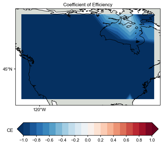
ce = LMRt.utils.coefficient_efficiency(tas_recon, tas_obs.value[mask])

[28]:

import seaborn as sns
import cartopy.crs as ccrs
import cartopy.feature as cfeature
from cartopy.mpl.ticker import LongitudeFormatter, LatitudeFormatter

fig = plt.figure(figsize=[8, 8])
ax = plt.subplot(projection=ccrs.PlateCarree(central_longitude=180))
ax.set_title('Coefficient of Efficiency')
# latlon_range = [0, 360, -90, 90]
latlon_range = [np.mod(-130, 360), np.mod(-70, 360), 30, 70]
transform=ccrs.PlateCarree()

ax.set_extent(latlon_range, crs=transform)
lon_formatter = LongitudeFormatter(zero_direction_label=False)
lat_formatter = LatitudeFormatter()
ax.xaxis.set_major_formatter(lon_formatter)
ax.yaxis.set_major_formatter(lat_formatter)

lon_ticks=[60, 120, 180, 240, 300]
lat_ticks=[-90, -45, 0, 45, 90]
lon_ticks = np.array(lon_ticks)
lat_ticks = np.array(lat_ticks)
lon_min, lon_max, lat_min, lat_max = latlon_range
mask_lon = (lon_ticks >= lon_min) & (lon_ticks <= lon_max)
mask_lat = (lat_ticks >= lat_min) & (lat_ticks <= lat_max)
ax.set_xticks(lon_ticks[mask_lon], crs=ccrs.PlateCarree())
ax.set_yticks(lat_ticks[mask_lat], crs=ccrs.PlateCarree())

levels = np.linspace(-1, 1, 21)
cbar_labels = np.linspace(-1, 1, 11)
cbar_title = 'CE'
extend = 'both'
cmap = 'RdBu_r'
cbar_pad=0.1
cbar_orientation='horizontal'
cbar_aspect=10
cbar_fraction=0.35
cbar_shrink=0.8
font_scale=1.5
land_color=sns.xkcd_rgb['light grey']
ocean_color=sns.xkcd_rgb['white']

ax.add_feature(cfeature.LAND, facecolor=land_color, edgecolor=land_color)
ax.add_feature(cfeature.OCEAN, facecolor=ocean_color, edgecolor=ocean_color)
ax.coastlines()
im = ax.contourf(ds['lon'].values, ds['lat'].values, ce, levels, transform=transform, cmap=cmap, extend=extend)
cbar = fig.colorbar(
    im, ax=ax, orientation=cbar_orientation, pad=cbar_pad, aspect=cbar_aspect,
    fraction=cbar_fraction, shrink=cbar_shrink)
cbar.set_ticks(cbar_labels)
cbar.ax.set_title(cbar_title, x=-0.05, y=0.1)

LMRt.showfig(fig)

../_images/tutorial_quickstart_recon_cropped_domain_29_0.png

[ ]: