A Pseudoproxy Experiment with GraphEM and pseudoPAGES2k
Expected time to run through: 30 mins
This tutorial demonstrates how to get a reconstruction using GraphEM, leveraging a simple pseudoproxy dataset generated from iCESM gridded, with the realistic spatial availability but full temporal avaiablity of the PAGES2kv2 dataset. The pseudoproxy are generated based on the original iCESM simulated tas plus white noise with SNR=10, using below code block:
Test data preparation
To go through this tutorial, please prepare test data following the steps:
Download the test case named “PPE_PAGES2k” with this link. Create a directory named “testcases” in the same directory where this notebook sits. Put the unzipped direcotry “PPE_PAGES2k” into “testcases”.
Below, we first load some useful packages, including our GraphEM.
[1]:
%load_ext autoreload
%autoreload 2

import LMRt
import GraphEM
import os
import numpy as np
import pandas as pd
import xarray as xr
import matplotlib.pyplot as  plt
Reconstruction
[2]:
job = GraphEM.ReconJob()
[3]:
job.load_configs('./testcases/PPE_PAGES2k/configs.yml', verbose=True)
GraphEM: job.load_configs() >>> loading reconstruction configurations from: ./testcases/PPE_PAGES2k/configs.yml
GraphEM: job.load_configs() >>> job.configs created
GraphEM: job.load_configs() >>> job.configs["job_dirpath"] = /Users/fzhu/Github/GraphEM/docsrc/tutorial/testcases/PPE_PAGES2k/recon
GraphEM: job.load_configs() >>> /Users/fzhu/Github/GraphEM/docsrc/tutorial/testcases/PPE_PAGES2k/recon created
{'anom_period': [1951, 1980],
 'calib_period': [1900, 2000],
 'job_dirpath': '/Users/fzhu/Github/GraphEM/docsrc/tutorial/testcases/PPE_PAGES2k/recon',
 'job_id': 'GraphEM_tutorial',
 'obs_path': {'tas': './data/obs/iCESM_ann.nc'},
 'obs_regrid_ntrunc': 21,
 'obs_varname': {'lat': 'lat', 'lon': 'lon', 'tas': 'tas'},
 'proxydb_path': './data/proxy/pseudoPAGES2k_dataset_tas_wn_SNR10_full_temporal_availability.pkl',
 'ptype_list': 'all',
 'recon_period': [1000, 2000]}
[4]:
job.load_proxydb(verbose=True)
GraphEM: job.load_proxydb() >>> job.configs["proxydb_path"] = /Users/fzhu/Github/GraphEM/docsrc/tutorial/testcases/PPE_PAGES2k/data/proxy/pseudoPAGES2k_dataset_tas_wn_SNR10_full_temporal_availability.pkl
GraphEM: job.load_proxydb() >>> 692 records loaded
GraphEM: job.load_proxydb() >>> job.proxydb created
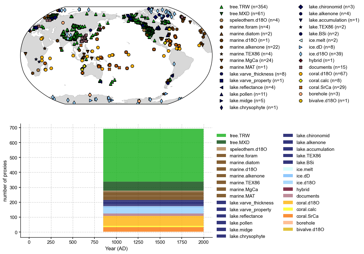
[5]:
fig, ax = job.proxydb.plot()
[6]:
job.load_obs(verbose=True)
print(job.obs)
GraphEM: job.load_obs() >>> loading instrumental observation fields from: {'tas': '/Users/fzhu/Github/GraphEM/docsrc/tutorial/testcases/PPE_PAGES2k/data/obs/iCESM_ann.nc'}
GraphEM: job.load_obs() >>> job.obs created
Dataset Overview
-----------------------

     Name:  tas
   Source:  /Users/fzhu/Github/GraphEM/docsrc/tutorial/testcases/PPE_PAGES2k/data/obs/iCESM_ann.nc
    Shape:  time:1156, lat:96, lon:144
[7]:
# regrid obs to make the problem size smaller
job.regrid_obs(verbose=True)
LMRt: job.regrid_obs() >>> regridded obs
Dataset Overview
-----------------------

     Name:  tas
   Source:  /Users/fzhu/Github/GraphEM/docsrc/tutorial/testcases/PPE_PAGES2k/data/obs/iCESM_ann.nc
    Shape:  time:1156, lat:22, lon:33
LMRt: job.regrid_obs() >>> job.obs updated
Since the loaded iCESM simulation and the pseudoproxy dataset are already annualized, we can skip the .seasonalize() steps and run .prep_data() directly.
[8]:
job.prep_data(verbose=True)
GraphEM: job.prep_data() >>> job.recon_time created
GraphEM: job.prep_data() >>> job.calib_time created
GraphEM: job.prep_data() >>> job.calib_idx created
GraphEM: job.prep_data() >>> job.temp created
GraphEM: job.prep_data() >>> job.df_proxy created
GraphEM: job.prep_data() >>> job.proxy created
GraphEM: job.prep_data() >>> job.lonlat created
[9]:
job.df_proxy
[9]:
| NAm_153 | Asi_245 | NAm_165 | Asi_178 | Asi_174 | Eur_016 | Asi_198 | NAm_145 | Arc_070 | Arc_071 | ... | Asi_119 | Ocn_153 | NAm_074 | Asi_026 | Ocn_169 | Asi_201 | Asi_179 | Arc_014 | Ocn_071 | Ocn_072 | |
|---|---|---|---|---|---|---|---|---|---|---|---|---|---|---|---|---|---|---|---|---|---|
| 1000.0 | 2.049447 | 1.206348 | -0.028154 | 0.354423 | 0.164291 | 0.700894 | 0.420136 | 1.610386 | 1.250028 | 1.241505 | ... | 0.828330 | 0.074526 | 1.969163 | 0.165617 | 0.331053 | -0.578854 | 0.188152 | 1.255906 | 0.304311 | 0.425676 |
| 1001.0 | 0.014990 | 0.708525 | 0.246777 | -0.057988 | -0.127694 | -0.077910 | 0.477898 | -1.579350 | -1.453855 | 1.689047 | ... | 0.986828 | -0.319637 | 1.589055 | 0.146957 | -0.345228 | -0.449773 | 0.128710 | 1.697772 | -0.457480 | -0.352040 |
| 1002.0 | -1.114598 | -0.355595 | -0.903415 | -0.370463 | -0.170471 | 0.018887 | 0.820904 | 0.335598 | 0.658790 | -1.006825 | ... | -0.571258 | -0.268028 | -2.308910 | 0.313561 | -0.265528 | -0.357028 | 0.152346 | -0.037280 | -0.357438 | -0.312209 |
| 1003.0 | 0.921028 | 0.761262 | -0.241008 | -0.612394 | -0.198821 | 0.600541 | 0.038012 | 1.649567 | 0.484537 | -0.694430 | ... | 0.332292 | 0.469818 | 1.270690 | -0.172501 | 0.210101 | -0.619913 | -0.157362 | -0.393430 | 0.248620 | 0.292726 |
| 1004.0 | 0.292958 | -0.005126 | 0.781568 | -0.169216 | 0.314034 | -0.194410 | 0.990756 | -0.391326 | -1.263733 | 1.176845 | ... | 0.160528 | -0.084175 | 0.971972 | 0.342813 | -0.134291 | 1.254460 | 0.379938 | 1.061491 | -0.126194 | -0.164533 |
| ... | ... | ... | ... | ... | ... | ... | ... | ... | ... | ... | ... | ... | ... | ... | ... | ... | ... | ... | ... | ... | ... |
| 1996.0 | 0.596161 | 0.397911 | -0.213472 | -0.375964 | 0.110367 | -0.175807 | 1.092398 | 2.554041 | 2.983670 | -0.233084 | ... | 0.086505 | 0.938570 | -0.516218 | 0.099238 | 0.489292 | 0.470537 | -0.122144 | -0.671030 | 0.416049 | 0.440858 |
| 1997.0 | 0.708165 | -0.204674 | 0.940863 | -0.811482 | -0.402413 | 0.229789 | 1.386490 | 0.106067 | -0.278486 | -0.677213 | ... | -0.236382 | 0.109457 | -0.916285 | -0.319777 | -0.009780 | 0.513189 | -0.707492 | -1.106939 | -0.174881 | -0.218647 |
| 1998.0 | 0.502749 | -0.240407 | 1.346490 | 0.595868 | 0.373318 | 0.085835 | 0.838359 | 0.328611 | 1.795783 | 2.179380 | ... | -0.454328 | 0.489631 | 0.177895 | 0.388473 | 0.009699 | 0.821627 | 0.307725 | 1.840054 | -0.005446 | 0.060198 |
| 1999.0 | 1.476074 | -0.101115 | 0.071156 | 0.010010 | 0.215712 | -0.452304 | -0.450495 | 2.144862 | 1.877791 | -0.456210 | ... | 0.340616 | 0.543951 | 0.590506 | 0.229498 | 0.373771 | 0.036311 | -0.097946 | -0.597891 | 0.509028 | 0.404405 |
| 2000.0 | -0.227916 | -0.418627 | 0.600212 | 1.064158 | 0.782957 | 1.423108 | 1.178986 | -0.110369 | 1.205325 | -0.306477 | ... | -0.156622 | 0.445898 | 0.449710 | 0.121985 | 0.304760 | 1.010402 | 0.186142 | 1.766690 | 0.499660 | 0.453703 |
1001 rows × 692 columns
[10]:
print(np.shape(job.temp))
print(np.shape(job.proxy))
print(np.shape(job.lonlat))
(1001, 726)
(1001, 692)
(1418, 2)
[11]:
job.save(verbose=True)
LMRt: job.save_job() >>> Prepration data saved to: /Users/fzhu/Github/GraphEM/docsrc/tutorial/testcases/PPE_PAGES2k/recon/job.pkl
LMRt: job.save_job() >>> job.configs["prep_savepath"] = /Users/fzhu/Github/GraphEM/docsrc/tutorial/testcases/PPE_PAGES2k/recon/job.pkl
[12]:
%%time

# need to remove G.pkl if the previous run is problematic
save_path = './testcases/PPE_PAGES2k/recon/G.pkl'
job.run_solver(save_path=save_path, verbose=True, distance=5e3)
Estimating graph using neighborhood method
Running GraphEM:

Iter     dXmis     rdXmis

001     0.0876     0.6708
002     0.4915     3.0970
003     0.1681     0.3053
004     0.1048     0.1687
005     0.0731     0.1107
006     0.0542     0.0788
007     0.0430     0.0606
008     0.0344     0.0474
009     0.0292     0.0395
010     0.0256     0.0341
011     0.0229     0.0300
012     0.0208     0.0270
013     0.0191     0.0245
014     0.0178     0.0226
015     0.0167     0.0210
016     0.0157     0.0197
017     0.0150     0.0186
018     0.0183     0.0226
019     0.0150     0.0184
020     0.0137     0.0167
021     0.0129     0.0157
022     0.0123     0.0149
023     0.0118     0.0142
024     0.0114     0.0137
025     0.0110     0.0132
026     0.0106     0.0127
027     0.0103     0.0123
028     0.0101     0.0120
029     0.0098     0.0116
030     0.0096     0.0113
031     0.0094     0.0110
032     0.0092     0.0108
033     0.0090     0.0105
034     0.0088     0.0103
035     0.0086     0.0101
036     0.0085     0.0099
037     0.0083     0.0097
038     0.0082     0.0096
039     0.0081     0.0094
040     0.0080     0.0092
041     0.0078     0.0091
042     0.0077     0.0090
043     0.0076     0.0088
044     0.0075     0.0087
045     0.0074     0.0086
046     0.0074     0.0085
047     0.0073     0.0084
048     0.0072     0.0083
049     0.0071     0.0082
050     0.0070     0.0081
051     0.0069     0.0080
052     0.0068     0.0079
053     0.0068     0.0078
054     0.0067     0.0077
055     0.0066     0.0076
056     0.0065     0.0075
057     0.0065     0.0074
058     0.0064     0.0073
059     0.0063     0.0072
060     0.0063     0.0072
061     0.0062     0.0071
062     0.0061     0.0070
063     0.0061     0.0069
064     0.0060     0.0069
065     0.0059     0.0068
066     0.0059     0.0067
067     0.0058     0.0066
068     0.0058     0.0066
069     0.0057     0.0065
070     0.0057     0.0065
071     0.0056     0.0064
072     0.0056     0.0063
073     0.0055     0.0063
074     0.0055     0.0062
075     0.0054     0.0062
076     0.0054     0.0061
077     0.0053     0.0060
078     0.0053     0.0060
079     0.0052     0.0059
080     0.0052     0.0059
081     0.0051     0.0058
082     0.0051     0.0058
083     0.0051     0.0058
084     0.0050     0.0057
085     0.0050     0.0057
086     0.0050     0.0056
087     0.0049     0.0056
088     0.0049     0.0055
089     0.0049     0.0055
090     0.0048     0.0055
091     0.0048     0.0054
092     0.0048     0.0054
093     0.0047     0.0054
094     0.0047     0.0053
095     0.0047     0.0053
096     0.0046     0.0052
097     0.0046     0.0052
098     0.0046     0.0052
099     0.0045     0.0051
100     0.0045     0.0051
101     0.0045     0.0051
102     0.0044     0.0050
103     0.0044     0.0050
GraphEM: job.run_solver() >>> job.G created and saved to: ./testcases/PPE_PAGES2k/recon/G.pkl
GraphEM: job.run_solver() >>> job.recon created
CPU times: user 1h 12min 41s, sys: 2min 26s, total: 1h 15min 8s
Wall time: 10min 39s
[13]:
job.save_recon('./testcases/PPE_PAGES2k/recon/recon.nc', verbose=True)
LMRt: job.save_recon() >>> Reconstruction saved to: ./testcases/PPE_PAGES2k/recon/recon.nc
Validation
[14]:
with xr.open_dataset('./testcases/PPE_PAGES2k/recon/recon.nc') as ds:
    print(ds)
<xarray.Dataset>
Dimensions:  (lat: 22, lon: 33, year: 1001)
Coordinates:
  * year     (year) int64 1000 1001 1002 1003 1004 ... 1996 1997 1998 1999 2000
  * lat      (lat) float64 -85.91 -77.73 -69.55 -61.36 ... 69.55 77.73 85.91
  * lon      (lon) float64 0.0 10.91 21.82 32.73 ... 316.4 327.3 338.2 349.1
Data variables:
    recon    (year, lat, lon) float64 ...
[15]:
mask = (job.obs.fields['tas'].time >= 1000) & (job.obs.fields['tas'].time <= 2000)
target = job.obs.fields['tas'].value[mask]
print(np.shape(target))
(1001, 22, 33)
Mean Statistics
[16]:
nt = np.size(ds['year'])
temp_r = job.recon.reshape((nt, -1))
V = GraphEM.solver.verif_stats(temp_r, target.reshape((nt, -1)), job.calib_idx)
print(V)
Mean MSE = 0.5291, Mean RE = 0.1882, Mean CE = -0.0223, Mean R2 = 0.3907
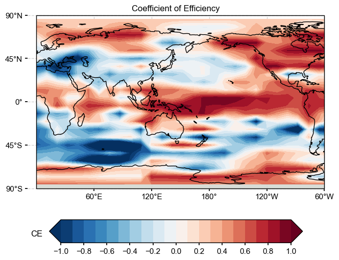
Map of CE
[17]:
ce = LMRt.utils.coefficient_efficiency(target, ds['recon'])
print(np.shape(ce))
(22, 33)
[18]:
import seaborn as sns
import cartopy.crs as ccrs
import cartopy.feature as cfeature
from cartopy.mpl.ticker import LongitudeFormatter, LatitudeFormatter

fig = plt.figure(figsize=[8, 8])
ax = plt.subplot(projection=ccrs.PlateCarree(central_longitude=180))
ax.set_title('Coefficient of Efficiency')
latlon_range = [0, 360, -90, 90]
transform=ccrs.PlateCarree()

ax.set_extent(latlon_range, crs=transform)
lon_formatter = LongitudeFormatter(zero_direction_label=False)
lat_formatter = LatitudeFormatter()
ax.xaxis.set_major_formatter(lon_formatter)
ax.yaxis.set_major_formatter(lat_formatter)

lon_ticks=[60, 120, 180, 240, 300]
lat_ticks=[-90, -45, 0, 45, 90]
lon_ticks = np.array(lon_ticks)
lat_ticks = np.array(lat_ticks)
lon_min, lon_max, lat_min, lat_max = latlon_range
mask_lon = (lon_ticks >= lon_min) & (lon_ticks <= lon_max)
mask_lat = (lat_ticks >= lat_min) & (lat_ticks <= lat_max)
ax.set_xticks(lon_ticks[mask_lon], crs=ccrs.PlateCarree())
ax.set_yticks(lat_ticks[mask_lat], crs=ccrs.PlateCarree())

levels = np.linspace(-1, 1, 21)
cbar_labels = np.linspace(-1, 1, 11)
cbar_title = 'CE'
extend = 'both'
cmap = 'RdBu_r'
cbar_pad=0.1
cbar_orientation='horizontal'
cbar_aspect=10
cbar_fraction=0.35
cbar_shrink=0.8
font_scale=1.5
land_color=sns.xkcd_rgb['light grey']
ocean_color=sns.xkcd_rgb['white']

ax.add_feature(cfeature.LAND, facecolor=land_color, edgecolor=land_color)
ax.add_feature(cfeature.OCEAN, facecolor=ocean_color, edgecolor=ocean_color)
ax.coastlines()
im = ax.contourf(ds['lon'].values, ds['lat'].values, ce, levels, transform=transform, cmap=cmap, extend=extend)
cbar = fig.colorbar(
    im, ax=ax, orientation=cbar_orientation, pad=cbar_pad, aspect=cbar_aspect,
    fraction=cbar_fraction, shrink=cbar_shrink)
cbar.set_ticks(cbar_labels)
cbar.ax.set_title(cbar_title, x=-0.05, y=0.1)

LMRt.showfig(fig)
/Users/fzhu/Apps/miniconda3/envs/LMRt/lib/python3.8/site-packages/cartopy/mpl/geoaxes.py:834: UserWarning: Attempting to set identical left == right == -180.0 results in singular transformations; automatically expanding.
  self.set_xlim([x1, x2])
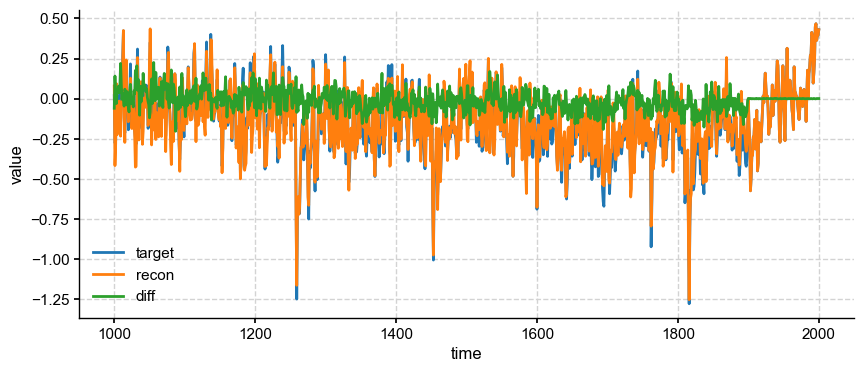
Mean timeseries
[19]:
import pyleoclim as pyleo
[20]:
def geo_mean(field, lat):
    m = np.average(
        np.average(field, axis=-1), axis=-1, weights=np.cos(np.deg2rad(lat))
    )
    return m
[21]:
m_target = geo_mean(target, job.obs.fields['tas'].lat)
ts_target = pyleo.Series(time=np.arange(1000, 2001), value=m_target)

m_recon = geo_mean(ds['recon'].values, ds['lat'].values)
ts_recon = pyleo.Series(time=ds['year'].values, value=m_recon)

fig, ax = ts_target.plot(mute=True, label='target')
ts_recon.plot(ax=ax, label='recon')
ax.plot(ds['year'].values, m_target-m_recon, label='diff')
ax.legend()
pyleo.showfig(fig)
[ ]: