A Pseudoproxy Experiment with GraphEM

Expected time to run through: 10 mins

This tutorial demonstrates how to get a reconstruction using GraphEM, leveraging a simple pseudoproxy dataset generated from a subset of iCESM gridded dataset. The pseudoproxy are generated based on the original iCESM simulated tas plus white noise with SNR=1, using below code block:

# gen pseudoproxy

SNR = 1

pp = np.copy(tas_sub)
nt, nlat, nlon = np.shape(pp)

k = 0
for i in range(nlat):
    for j in range(nlon):
        tas_std = np.std(tas_sub[:,i,j])
        noise_std = tas_std / SNR

        np.random.seed(k)
        pp[:,i,j] += np.random.normal(0, noise_std, size=nt)

        k += 1

Test data preparation

To go through this tutorial, please prepare test data following the steps:

Download the test case named “PPE” with this link. Create a directory named “testcases” in the same directory where this notebook sits. Put the unzipped direcotry “PPE” into “testcases”.

Below, we first load some useful packages, including our GraphEM.

[1]:

%load_ext autoreload
%autoreload 2

import LMRt
import GraphEM
import os
import numpy as np
import pandas as pd
import xarray as xr
import matplotlib.pyplot as  plt

Reconstruction

[2]:

job = GraphEM.ReconJob()

[3]:

job.load_configs('./testcases/PPE/configs.yml', verbose=True)

GraphEM: job.load_configs() >>> loading reconstruction configurations from: ./testcases/PPE/configs.yml
GraphEM: job.load_configs() >>> job.configs created
GraphEM: job.load_configs() >>> job.configs["job_dirpath"] = /Users/fzhu/Github/GraphEM/docsrc/tutorial/testcases/PPE/recon
GraphEM: job.load_configs() >>> /Users/fzhu/Github/GraphEM/docsrc/tutorial/testcases/PPE/recon created
{'anom_period': [1951, 1980],
 'calib_period': [1750, 1849],
 'job_dirpath': '/Users/fzhu/Github/GraphEM/docsrc/tutorial/testcases/PPE/recon',
 'job_id': 'LMRt_quickstart',
 'obs_path': {'tas': './data/obs/iCESM_subset.nc'},
 'obs_varname': {'lat': 'lat', 'lon': 'lon', 'tas': 'tas'},
 'proxydb_path': './data/proxy/pseudoproxy_dataset.pkl',
 'ptype_list': ['coral.d18O'],
 'recon_period': [850, 1849]}

[4]:

job.load_proxydb(verbose=True)

GraphEM: job.load_proxydb() >>> job.configs["proxydb_path"] = /Users/fzhu/Github/GraphEM/docsrc/tutorial/testcases/PPE/data/proxy/pseudoproxy_dataset.pkl
GraphEM: job.load_proxydb() >>> 100 records loaded
GraphEM: job.load_proxydb() >>> job.proxydb created

[5]:

job.filter_proxydb(verbose=True)

GraphEM: job.filter_proxydb() >>> filtering proxy records according to: ['coral.d18O']
GraphEM: job.filter_proxydb() >>> 100 records remaining

[6]:

job.load_obs(verbose=True)

GraphEM: job.load_obs() >>> loading instrumental observation fields from: {'tas': '/Users/fzhu/Github/GraphEM/docsrc/tutorial/testcases/PPE/data/obs/iCESM_subset.nc'}
Time axis not overlap with the reference period [1951, 1980]; use its own time period as reference [850.00, 1849.00].
GraphEM: job.load_obs() >>> job.obs created

[7]:

print(job.obs)

Dataset Overview
-----------------------

     Name:  tas
   Source:  /Users/fzhu/Github/GraphEM/docsrc/tutorial/testcases/PPE/data/obs/iCESM_subset.nc
    Shape:  time:1000, lat:10, lon:10

Since the loaded iCESM simulation and the pseudoproxy dataset are already annualized, we can skip the .seasonalize() steps and run .prep_data() directly.

[8]:

job.prep_data(verbose=True)

GraphEM: job.prep_data() >>> job.recon_time created
GraphEM: job.prep_data() >>> job.calib_time created
GraphEM: job.prep_data() >>> job.calib_idx created
GraphEM: job.prep_data() >>> job.temp created
GraphEM: job.prep_data() >>> job.df_proxy created
GraphEM: job.prep_data() >>> job.proxy created
GraphEM: job.prep_data() >>> job.lonlat created

[9]:

job.df_proxy

[9]:

	pp_000	pp_001	pp_002	pp_003	pp_004	pp_005	pp_006	pp_007	pp_008	pp_009	...	pp_090	pp_091	pp_092	pp_093	pp_094	pp_095	pp_096	pp_097	pp_098	pp_099
850.0	300.751783	300.699385	299.718651	300.717691	299.793416	299.939352	299.472350	300.551011	299.553801	299.413664	...	299.249156	299.027787	299.182322	299.526141	299.161496	298.628304	298.802706	298.107757	298.818966	298.544758
851.0	300.496749	300.009875	300.193606	300.365040	300.347096	299.853183	300.380611	299.650771	300.502845	299.614965	...	299.103565	298.778987	299.141563	299.335989	299.410467	298.670001	298.838717	298.689713	299.370283	299.494514
852.0	300.902166	300.334244	299.602851	300.671260	300.102458	301.886292	300.641600	300.462630	299.210613	299.595454	...	299.289380	299.249218	299.134434	299.942948	298.988984	299.277950	298.905532	298.840735	299.414093	299.140887
853.0	301.729269	300.347924	301.572955	299.850196	301.104819	300.567805	300.145062	300.817268	299.709402	300.448917	...	299.573146	299.649931	298.838391	299.710779	300.040319	299.609617	299.473822	299.656169	299.019936	299.719184
854.0	301.378359	300.997108	299.769165	300.429641	300.280460	300.495473	298.998074	299.858000	298.895901	299.967372	...	300.078972	300.040279	299.551374	300.088576	298.790187	299.790875	299.441056	299.184892	299.035147	299.345002
...	...	...	...	...	...	...	...	...	...	...	...	...	...	...	...	...	...	...	...	...	...
1845.0	300.370235	300.113197	300.144971	299.726555	299.921271	300.382517	299.913085	299.789860	299.300107	299.261318	...	299.482236	299.063248	299.152310	298.784250	298.994037	298.300974	299.091353	298.409069	298.584221	298.305443
1846.0	299.985712	298.994364	300.207191	299.883894	300.684450	300.181971	300.745885	299.919197	298.775608	299.324020	...	299.544706	299.056843	299.350263	299.165946	299.459059	299.227588	299.156746	299.367724	299.111197	298.400678
1847.0	300.292753	300.177510	300.033955	300.236235	299.559872	299.877648	299.141349	299.497879	299.952182	299.577197	...	299.724081	300.424495	299.179294	299.375003	299.475237	299.947260	300.159204	299.223168	299.384652	299.483399
1848.0	299.823016	300.400975	300.223044	300.913630	300.261049	300.159285	299.311807	299.449942	299.660750	298.979497	...	299.829125	299.592597	300.013318	299.155958	299.107011	299.086289	299.878042	299.307766	299.593688	298.706442
1849.0	300.161352	300.159181	300.246488	299.820504	299.517483	299.951131	299.332212	299.316922	299.630661	299.881939	...	299.587589	298.878817	298.997188	298.895755	299.134630	299.284257	299.369434	299.400078	299.026855	299.096824

1000 rows × 100 columns

[10]:

print(np.shape(job.temp))
print(np.shape(job.proxy))
print(np.shape(job.lonlat))

(1000, 100)
(1000, 100)
(200, 2)

[11]:

job.save(verbose=True)

LMRt: job.save_job() >>> Prepration data saved to: /Users/fzhu/Github/GraphEM/docsrc/tutorial/testcases/PPE/recon/job.pkl
LMRt: job.save_job() >>> job.configs["prep_savepath"] = /Users/fzhu/Github/GraphEM/docsrc/tutorial/testcases/PPE/recon/job.pkl

[12]:

%%time

save_path = './testcases/PPE/recon/G.pkl'
job.run_solver(save_path=save_path, verbose=True)

Estimating graph using neighborhood method
Running GraphEM:

Iter     dXmis     rdXmis

001     0.0514     3.1516
002     0.4586     8.5151
003     0.0562     0.1136
004     0.0292     0.0566
005     0.0149     0.0287
006     0.0123     0.0235
007     0.0107     0.0203
008     0.0092     0.0174
009     0.0081     0.0152
010     0.0073     0.0137
011     0.0067     0.0126
012     0.0063     0.0117
013     0.0059     0.0110
014     0.0055     0.0103
015     0.0053     0.0098
016     0.0050     0.0094
017     0.0048     0.0090
018     0.0047     0.0087
019     0.0045     0.0084
020     0.0044     0.0082
021     0.0043     0.0079
022     0.0041     0.0077
023     0.0040     0.0075
024     0.0039     0.0072
025     0.0038     0.0070
026     0.0036     0.0068
027     0.0035     0.0065
028     0.0034     0.0063
029     0.0033     0.0061
030     0.0032     0.0059
031     0.0031     0.0057
032     0.0030     0.0055
033     0.0029     0.0053
034     0.0028     0.0051
035     0.0027     0.0050
GraphEM: job.run_solver() >>> job.G created and saved to: ./testcases/PPE/recon/G.pkl
GraphEM: job.run_solver() >>> job.recon created
CPU times: user 18.2 s, sys: 3.42 s, total: 21.6 s
Wall time: 3.45 s

[13]:

job.save_recon('./testcases/PPE/recon/recon.nc', verbose=True)

LMRt: job.save_recon() >>> Reconstruction saved to: ./testcases/PPE/recon/recon.nc

Validation

[14]:

with xr.open_dataset('./testcases/PPE/recon/recon.nc') as ds:
    print(ds)

<xarray.Dataset>
Dimensions:  (lat: 10, lon: 10, year: 1000)
Coordinates:
  * year     (year) int64 850 851 852 853 854 855 ... 1845 1846 1847 1848 1849
  * lat      (lat) float32 -4.737 -2.842 -0.9474 0.9474 ... 8.526 10.42 12.32
  * lon      (lon) float32 162.5 165.0 167.5 170.0 ... 177.5 180.0 182.5 185.0
Data variables:
    recon    (year, lat, lon) float64 ...

[15]:

target = job.obs.fields['tas'].value

Mean Statistics

[76]:

nt = np.size(ds['year'])
temp_r = job.recon.reshape((nt, -1))
V = GraphEM.solver.verif_stats(temp_r,target.reshape((nt, -1)), job.calib_idx)
print(V)

Mean MSE = 0.0206, Mean RE = 0.9000, Mean CE = 0.8999, Mean R2 = 0.9022

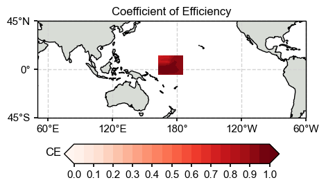
Map of CE

[16]:

ce = LMRt.utils.coefficient_efficiency(target, ds['recon'])
print(np.shape(ce))

(10, 10)

[73]:

import seaborn as sns
import cartopy.crs as ccrs
import cartopy.feature as cfeature
from cartopy.mpl.ticker import LongitudeFormatter, LatitudeFormatter

fig = plt.figure(figsize=[5, 5])
ax = plt.subplot(projection=ccrs.PlateCarree(central_longitude=180))
ax.set_title('Coefficient of Efficiency')
latlon_range = [50, 300, -45, 45]
transform=ccrs.PlateCarree()

ax.set_extent(latlon_range, crs=transform)
lon_formatter = LongitudeFormatter(zero_direction_label=False)
lat_formatter = LatitudeFormatter()
ax.xaxis.set_major_formatter(lon_formatter)
ax.yaxis.set_major_formatter(lat_formatter)

lon_ticks=[60, 120, 180, 240, 300]
lat_ticks=[-90, -45, 0, 45, 90]
lon_ticks = np.array(lon_ticks)
lat_ticks = np.array(lat_ticks)
lon_min, lon_max, lat_min, lat_max = latlon_range
mask_lon = (lon_ticks >= lon_min) & (lon_ticks <= lon_max)
mask_lat = (lat_ticks >= lat_min) & (lat_ticks <= lat_max)
ax.set_xticks(lon_ticks[mask_lon], crs=ccrs.PlateCarree())
ax.set_yticks(lat_ticks[mask_lat], crs=ccrs.PlateCarree())

levels = np.linspace(0, 1, 21)
cbar_labels = np.linspace(0, 1, 11)
cbar_title = 'CE'
extend = 'both'
cmap = 'Reds'
cbar_pad=0.1
cbar_orientation='horizontal'
cbar_aspect=10
cbar_fraction=0.35
cbar_shrink=0.8
font_scale=1.5
land_color=sns.xkcd_rgb['light grey']
ocean_color=sns.xkcd_rgb['white']

ax.add_feature(cfeature.LAND, facecolor=land_color, edgecolor=land_color)
ax.add_feature(cfeature.OCEAN, facecolor=ocean_color, edgecolor=ocean_color)
ax.coastlines()
im = ax.contourf(ds['lon'].values, ds['lat'].values, ce, levels, transform=transform, cmap=cmap, extend=extend)
cbar = fig.colorbar(
    im, ax=ax, orientation=cbar_orientation, pad=cbar_pad, aspect=cbar_aspect,
    fraction=cbar_fraction, shrink=cbar_shrink)
cbar.set_ticks(cbar_labels)
cbar.ax.set_title(cbar_title, x=-0.05, y=0.1)

LMRt.showfig(fig)

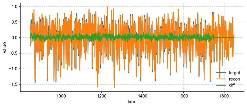
../_images/tutorial_quickstart_ppe_25_0.png

Mean timeseries

[79]:

import pyleoclim as pyleo

[81]:

def geo_mean(field, lat):
    m = np.average(
        np.average(field, axis=-1), axis=-1, weights=np.cos(np.deg2rad(lat))
    )
    return m

[87]:

m_target = geo_mean(job.obs.fields['tas'].value, job.obs.fields['tas'].lat)
ts_target = pyleo.Series(time=job.obs.fields['tas'].time, value=m_target)

m_recon = geo_mean(ds['recon'].values, ds['lat'].values)
ts_recon = pyleo.Series(time=ds['year'].values, value=m_recon)

fig, ax = ts_target.plot(mute=True, label='target')
ts_recon.plot(ax=ax, label='recon')
ax.plot(ds['year'].values, m_target-m_recon, label='diff')
ax.legend()
pyleo.showfig(fig)

../_images/tutorial_quickstart_ppe_29_0.png

[ ]: