Individual maps
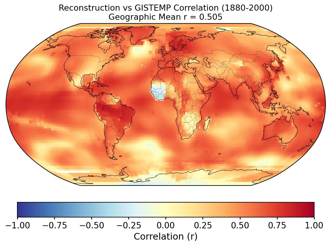
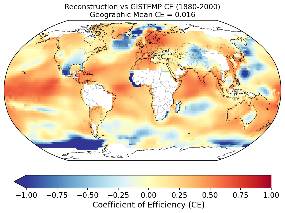
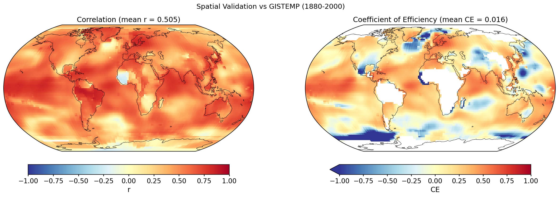
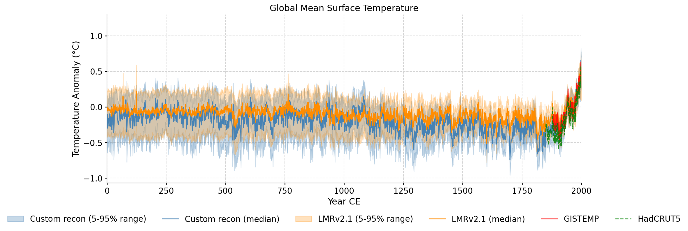
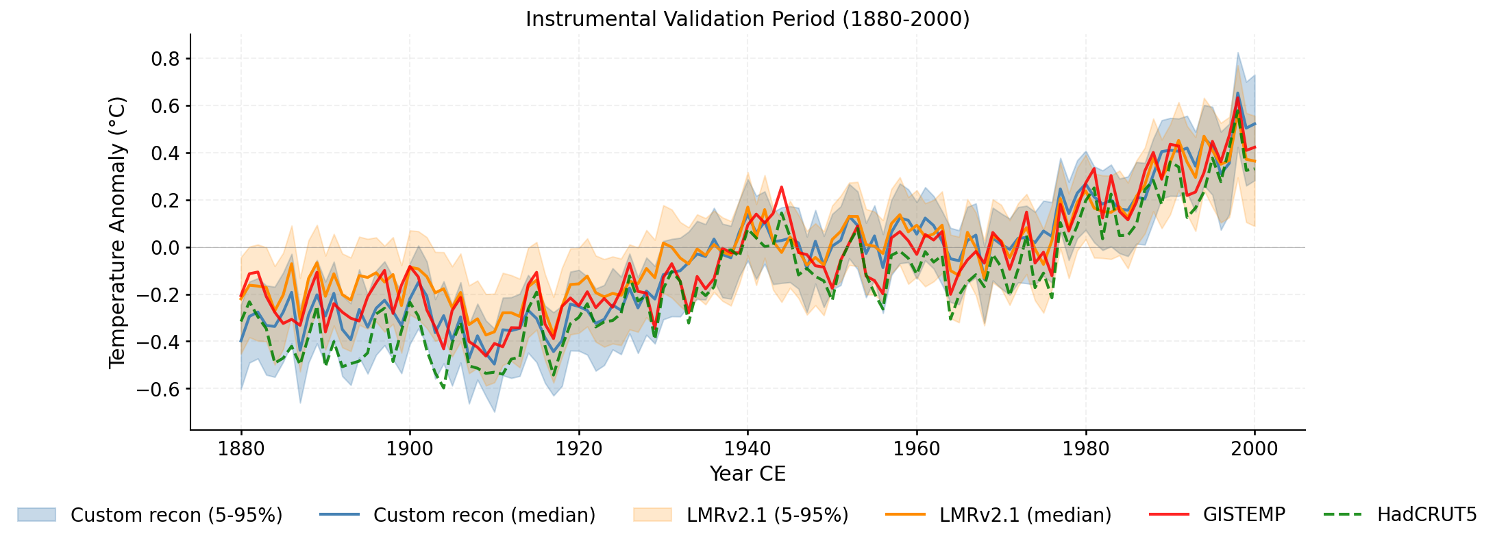
Validation of the custom LMR reconstruction against instrumental observations and the published LMRv2.1, following the methodology of PReSto2k validation.
Performance of the ensemble-median global mean surface temperature (GMST) against instrumental datasets over the validation window. Two metrics are reported for each reconstruction/reference pair.
Pearson correlation (R): linear association between the two time series. R measures pattern agreement but is insensitive to systematic offsets or amplitude errors.
Nash–Sutcliffe Coefficient of Efficiency
(CE; Nash & Sutcliffe, 1970):
CE = 1 − Σ(y −
Ŷ)2 /
Σ(y − Ȳ)2,
where y is the observation, Ŷ is the
reconstruction, and Ȳ is the mean of the observations
over the validation window.
CE captures pattern, amplitude, and bias simultaneously:
Reference datasets: GISTEMP (NASA GISS surface temperature analysis, ERSSTv4 ocean; data.giss.nasa.gov); HadCRUT5 (Met Office Hadley Centre / CRU analysis; metoffice.gov.uk); Consensus — the arithmetic mean of the instrumental datasets listed above, taken over the years where all inputs have data. This is not an authoritative product; it is a local summary used here to smooth between-dataset differences when evaluating the reconstruction.
| Reconstruction | Reference | R | CE |
|---|---|---|---|
| Custom Recon | GISTEMP | 0.9246 | 0.8296 |
| LMRv2.1 | GISTEMP | 0.9319 | 0.8329 |
| Custom Recon | HadCRUT5 | 0.9368 | 0.7355 |
| LMRv2.1 | HadCRUT5 | 0.9329 | 0.5648 |
| Custom Recon | Consensus | 0.9352 | 0.8257 |
| LMRv2.1 | Consensus | 0.9367 | 0.7336 |
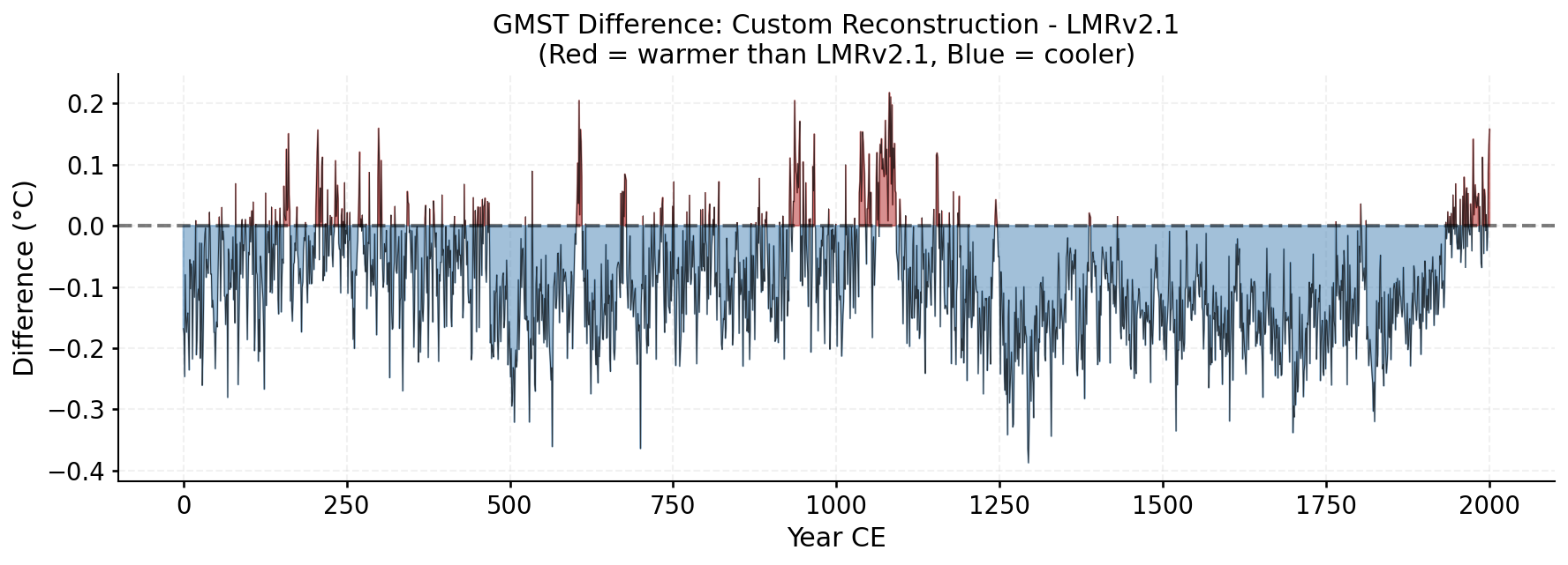
| Custom Recon | LMRv2.1 (0-2000) | 0.8067 | -0.8863 |
Grid-point R and CE between the custom reconstruction and GISTEMP over 1880–2000. Each cell's score is computed against its own 1951–1980 climatology (for anomalies) and its own time-series mean over the validation window (for the CE denominator); the geographic mean reported with each map is area-weighted.
Why the geographic-mean CE is so much lower than the GMST CE. The two numbers measure different things. At any single grid cell, most of the observed variance is local — weather noise, regional modes (ENSO, NAO, AMO, PDO) — which a paleoclimate reconstruction does not resolve. The reconstruction primarily captures the large-scale, slowly varying forced signal (volcanic, solar, anthropogenic), which is a small fraction of local variance. So per-cell CE is typically low or negative across much of the globe. When those cells are averaged into the global mean, the local noise averages towards zero and the forced signal dominates the residual variance, so the global-mean CE ends up much higher. In other words, the geographic mean of per-cell CE is not the CE of the geographic-mean time series — these are two different statistics and should not be expected to match.
Custom reconstruction ensemble spread compared against LMRv2.1, GISTEMP, and HadCRUT5.
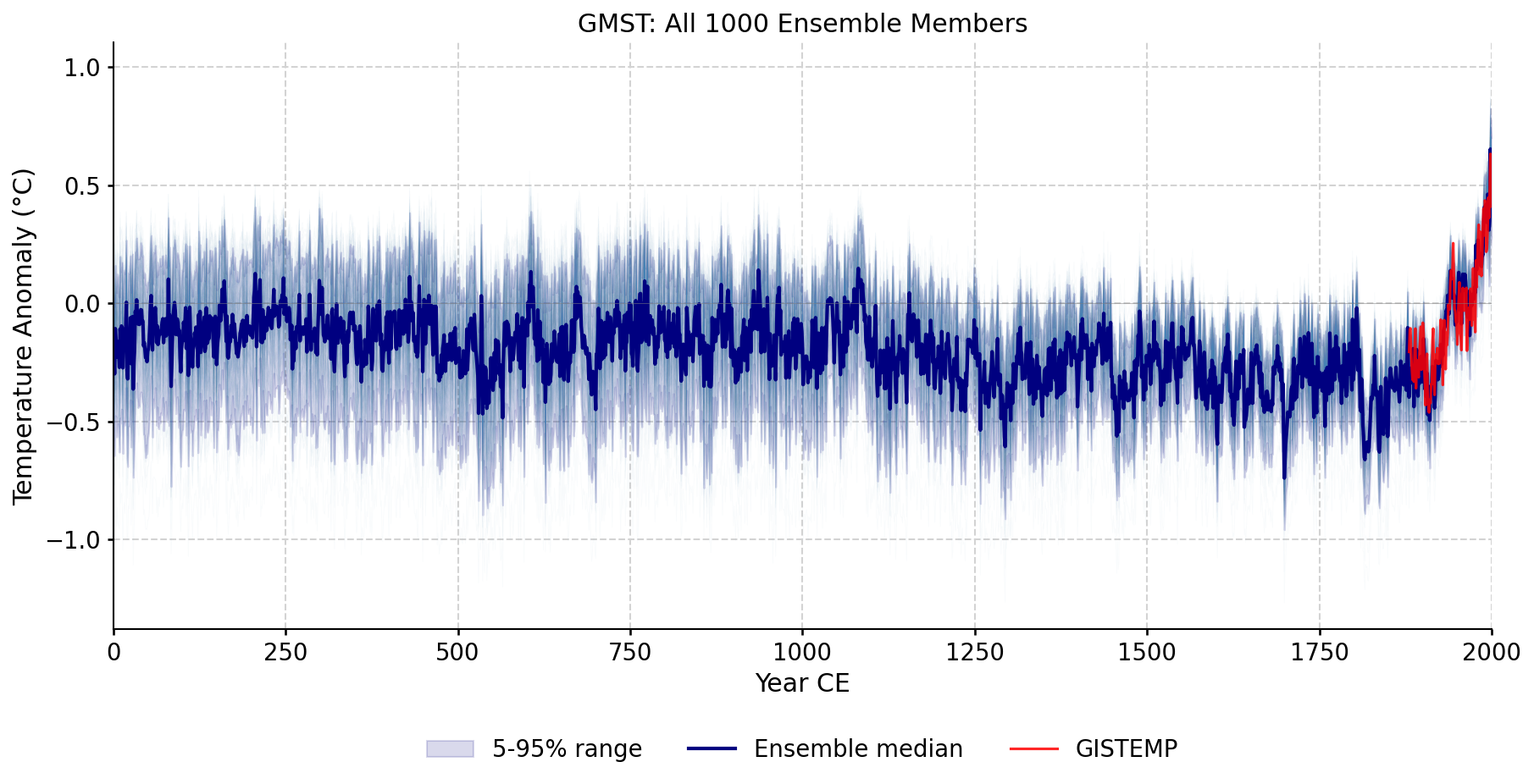
Every ensemble member plotted individually, showing the full spread of the reconstruction across all iterations and seeds.
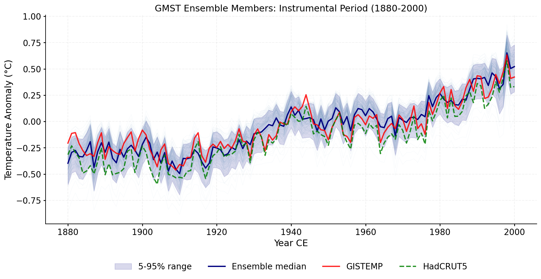
Zoomed view of ensemble members during the instrumental overlap period, with GISTEMP and HadCRUT5 overlaid.
Zoomed view of the validation period (1880-2000) with ensemble spread and all reference datasets.
Year-by-year difference between the custom reconstruction and LMRv2.1 ensemble medians. Red = warmer, Blue = cooler.